Introduction
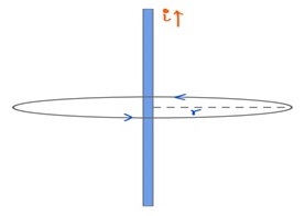
Ampere’s law placed a milestone for the development of Electrodynamics. Hans Oersted in 1920 performed a classic experiment with a compass needle and current carrying conductor. He observed that if there is no current in the wire then the compass needle always points towards the north pole. However, in the presence of current in the wire, the needle deflects in some direction. He found the direction of deflection is tangent to a circle i.e. Direction of magnetic field (Figure 1).
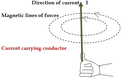
Fig-1: Direction of Magnetic field around a Current Carrying Wire
It established that current carrying wires produce a magnetic field around them. In principle we can always estimate the magnetic field due to current carrying cord using iot-savart’s law. To estimate the net magnetic field due to any current distribution, we first write the differential magnetic field (dB) ⃗ and then sum it over the whole distribution. But, what if we have a symmetry in our current distribution? Can we simplify our calculation? The answer is – Yes. Ampere’s law helps us to calculate magnetic fields.
Who was André-Marie Ampere?
André-Marie Ampère born in 1775 was a french Physicist and mathematician. He was a prodigy and started studying mathematics at the age of 12. Oersted’s discovery that magnetic fields are produced by electric current,attracted him towards this field. He carried forward the work of Oersted and demonstrated that current carrying wire repels or attracts each other. This repulsion or attraction depends upon the direction of current in the wire. He is famous for his well-known result called “Ampere’s Law”. In his honour, SI unit of current is named after him.
Explore our latest online courses and learn new skills at your own pace. Enroll and become a certified expert to boost your career.
Statement of Ampere’s Circuital Law
Ampere’s law can be stated in the following way – “The line integral of the force of field throughout any closed coil containing the steady current is proportional to the current passing through that coil.”
If there are numbers of currents passing through the loop then we will take the numerical sum of the currents enclose by the coil. The coil considered for the calculation is called “Amperian Loop or Amperian coil”.
Alternative Form of Ampere’s Circuital Law
Suppose there is a closed path C and net current passing through it is iencienc Then
∫B→.dl→=μ0ienc∫B→.dl→=μ0ienc
Let us analyse each term of this equation.
Line Integral of B→B→- we can divide loop into small vector elements dl→dl→.then
B→.dl→=BdlcosθB→.dl→=Bdlcosθ
Hence it is a product of the line element and tangent part of the magnetic field( Bcosθ) the loop.
Net current iencienc – We need to consider the algebraic sum of only those current elements which are passing through the loop.
From figure ienc=i1+i2ienc=i1+i2 only
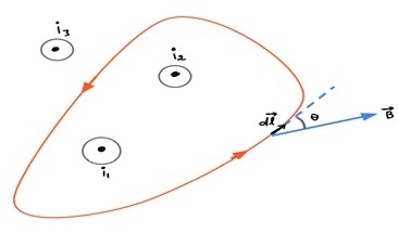
Direction of Integral – The direction of integral can be calculated using the Right-hand rule. If we curl our right hand pointing our fingers towards the direction of integration, then the outstretched thumb will point towards the positive direction of current.
Inconsistency of Ampere’s Circuital Law
Let us apply ampere’s law to a situation shown in the figure below. We have a capacitor and the conduction(conventional) current is denoted by icic. According to ampere’s law the integral B→.dl→B→.dl→ around the path should be equal to μ0iencμ0ienc
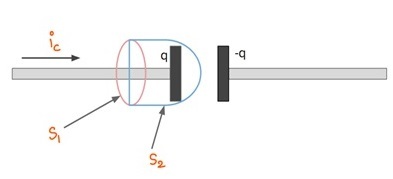
Here we take two surfaces. For surface S1:ienc=icS1:ienc=ic
For the surface S2S2 which is bulged out to right: ienc=0ienc=0 , since no current exists between the gaps of the capacitor.
Here B→.dl→B→.dl→ is zero and icic at the same time for the same path, which is contradictory.
Modified Ampere’s Circuital Law or Ampere – Maxwell’s Circuital Law
Maxwell modified the ampere’s law to remove this ambiguity by introducing a new term called “displacement current.’ It is defined as
id=ϵ0dΦEdtid=ϵ0dΦEdt
Where ΦEΦE is the electric flux through the surface given by ΦE=∫E→.dA−→ΦE=∫E→.dA→.
Hence the modified form of Ampere’s law or Ampere-Maxwell’s law is –
∫(B→).(dl→)=μ0(ic+id)=μ0ic+μ0ϵ0dΦEdt∫(B→).(dl→)=μ0(ic+id)=μ0ic+μ0ϵ0dΦEdt
Now we can solve the problem arising in the case of capacitors using Ampere-Maxwell law.
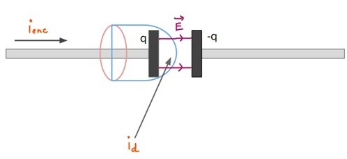
If we apply this law to surface S1:ienc=icS1:ienc=ic as usual
But for the surface S2S2 which is bulged out to right: ienc=0ienc=0 but id=ϵ0dΦEdtid=ϵ0dΦEdt since the electric field will be variable between the gaps of the capacitor.
Hence if there are time varying fields present inside the loop, we have to use Ampere-Maxwell’s Law to solve the problems.
Application of Ampere’s Circuital Law
We can use Ampere’s law to Variety of problems where Current distribution is symmetrical.
Let us consider a linear wire of radius R carrying current i. Let us apply Ampere’s law to estimate the magnetic field due to this wire at a distance r . (r>>R)
We can see that wire has a cylindrical symmetry. Using Right hand rule we can calculate the direction of B. It comes out to be tangent to every point of the Amperian loop and line element dl is parallel to the Amperian loop. It means B→B→ and dl→dl→ are parallel to each other.
Which means
B→.dl→=Bdlcosθ=Bdlcos0∘=BdlB→.dl→=Bdlcosθ=Bdlcos0∘=Bdl
Ampere’s Law
∫B→.dl→=∮B.dl=B∮dl=B.2Πr=μ0I∫B→.dl→=∮B.dl=B∮dl=B.2Πr=μ0I
Hence
B=μ0i2πrB=μ0i2πr
which is a well-known result and can be verified using Biot-savart’s law also.
Solved Examples
Example1: Find the value for B→.dl→B→.dl→ in surface 1 and 2.
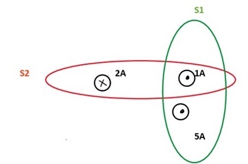
Ans: We can see from the figure that S1 contains two currents 1A and 5A.B→.dl→=65A.B→.dl→=6 S2 also contains two currents but one in a negative direction. B→.dl→=5−2=3B→.dl→=5−2=3
Example 2: A long straight wire of radius R=2cm is carrying a current 10A. Find the magnetic field 8cm away from it?
We have derived the equation for the magnetic field due to straight wire. We can directly use it here.
B=μ0i2Πr=4Π×107×102Π×8×10−2=20×10−58=2.5×10⁻⁵TeslaB=μ0i2Πr=4Π×107×102Π×8×10−2=20×10−58=2.5×10⁻⁵Tesla
Conclusion
We can simplify our estimation of force of field due to current distributions using Ampere’s law. But it can only be used if there is some symmetry in the system. If there is some source of varying electric field inside the loop then Ampere’s law fails to give any reasonable result. Maxwell modified this law for such cases and introduced the concept of Displacement current. Which can be demonstrated using the case of capacitors. We can use Ampere’s law to estimate force of field due to linear current carrying wire and it comes out to be inversely proportional to the distance at which we are calculating the field
Leave a Reply